One of the necessary systems in game AI is to be able to plan an agent’s path from A to B. For characters and human-like agents this is now routine, with game engines including built-in functionality for on-the-fly path-planning in a dynamic world. These systems start to reach their limits, however, when used with agents such as cars, boats, horses (and other animals). These agents have motion-constraints, which either prevent them changing their orientation on the spot (cars), or they need to slow down in order to change direction (horses, boats, skiers etc.).
The easiest way to produce paths for such agents is to perform a regular spatial search (e.g. using hierarchical A*) and then construct a curve through the resulting points. If the curves intersect obstacles, or don’t meet the motion constraints, some iterative adjustments can be made to refine them. This is the approach we use in 3D, and tends to work well in open game environments where there is space for adjustment. The downsides of this approach are that it may fail to find a path (if the path from the discrete search was not compatible with the motion constraints), or that the path is unnecessarily tight (if there was an alternative quick, smooth path that was ignored due to its length).
Discretising orientations as an extra dimension
A more complete solution to this problem is to include the kinematic constraints in the search, that is to say construct the search graph not only in (x,y), but to add a dimension for orientation, i.e. every graph node corresponds to an (x,y,angle). Other constraints such as speed could also be added, though we need to be a little bit cautious that search time is exponential in the number of dimensions, so if you start adding all your constraints you might only be able to do a single pathfind per game(!)
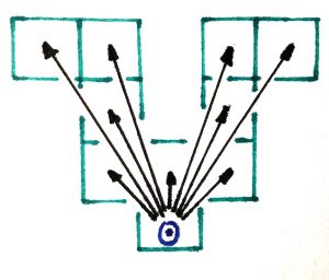
Once you have chosen a discretisation you then need to describe which transitions are allowed, that is to say, if you are at one spatial position facing in one direction, which other spatial positions and facing directions are you allowed to move to. Pictured right is the directions when moving up to 3 cells on a discrete grid, between -45 and +45 degrees.

A good direction discretisation is a trade-off between resolving the minimum turning circle of the agent over the cell size (i.e. so that orientations are fine enough to be changed between adjacent cells), and not having so many orientations that the pathfinds become very expensive. The final consideration is to have enough orientations to discretise the metric (discussed in the next section), though this is usually only a problem for agents with very small turning circles.
A* with a metric that penalises tight turns
Once you have described the allowed transitions, we then need to define the cost of our path. An agent typically turns with wider arcs than the minimum turning circle, since doing so would require travelling at a very low speed (i.e. not to slip). This can be encouraged in the search metric, which is the objective function that our graph search algorithm (in our case A*) will attempt to minimise.
In order to discourage tight turns we add a penalty for each discrete turn that the agents make. The size of this penalty is chosen to correspond to some distance (i.e. the usual cost function) and reduces as the distance from the previous turn increases, so the agent will try to maintain curves larger than some “ideal” radius. Taking a car for example, then this ideal radius could be the turning radius at maximum speed.

Whilst the cost function can, in principle, be any function of a sequence of nodes (i.e. description of a complete path), it is usually desirable to have a metric where the partial paths can be ranked. This allows A* to pick the lower cost partial path for each node it reaches and discard the others. This somewhat complicates metrics like integrated acceleration, or non-monotonic cost-functions.
Other general considerations of A* also apply, where cost functions with extreme values are usually to be avoided (since the path-find will usually run out resources before exploration, so those connections will never be searched, even if they were necessary).
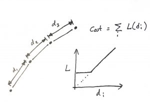
In Mercuna Ground Navigation we attempt to balance these considerations, and our metric is the sum of a function of the distance of each straight-line segment, with that function pictured right. This penalises very short distances between turns, and encourages longer wider turns. We also include an additional term for penalising steep slopes (not shown).
From line segments to smooth curves
The resulting path from an A* search will be a route both discrete in space (passing through cells) and in angle (our orientation discretisation), resulting in a zig-zag path through the grid. Our actual problem, however, both has more freedom (we can move the path continuously in space), and is more restrictive (we need smooth curves, rather than transitions between adjacent angles).

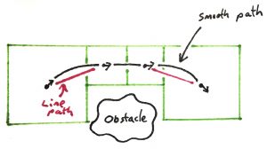
In order to construct the smooth path we create a sequence of parabolic segments (splines) which match the end points and (average) tangents of the straight line segments, pictured. These curves will not always avoid geometry (that was only guaranteed for straight lines), but we can iteratively adjust the parameters of the curves until they fit.
One final improvement that we make is to go back to the continuous cost function (usually the time to traverse the path), and attempt to smooth out any turns that were unnecessarily introduced by discretisation onto a finite graph.
Summary
Robust pathfinding for vehicles and animals requires significantly more machinery than 2D character navigation. Here we’ve tried to describe some of the core ingredients upon which Mercuna’s kinematic pathfinder is built, and hopefully it gives you an outline of what is going on “under the hood”. We are excited to make Mercuna Ground Navigation available to developers and look forward to seeing the games they build with it. Download our evaluation to try it out.


